Content Reconstruction

If you’re reading this, I’m assuming that you’ve read the paper Image Style Transfer Using Convolutional Neural Networks and have some familiarity with it.

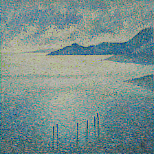
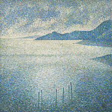
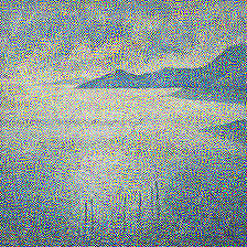
Here is the image I’ll be working with for this post:

The focus of this post is on the Content Representation/Reconstruction section of the paper, Section 2.1 to be precise. The authors use the title Content Representation yet I’ve also included the word Reconstruction here since that’s what they did in Figure 1 and what I’ve attempted to do on my own as well. Throughout this article, I’m essentially describing building this notebook.

Throughout working on this (sub) project, I ran into lots of issues. There’s so much that happens between the description in the paper and a fully-fledged implementation that I’ve never had to consider before. While I don’t consider what I’ve done to be exhausitive, even just considering Content Representation, it’s quite thorough and I’ve decided to talk about the most significant gotchas I ran into. As some of these might be obvious to some of you, I’ve shifted the gotchas into separate posts and throughout this post I’ll explicitly link to those mini write-ups. I hope that they help you avoid sinking as much time as I did into these issues.

So at the very start of the project, I wrote up the following TODO list:

• Obtain a pre-trained vgg-19 network.
• Push an image through an extract the outputs from the layers:
• Conv1_2
• Conv2_2
• Conv3_2
• Conv4_2
• Conv5_2
• Push white noise through and extract outputs from the same layer.
• Calculate the loss between the output from the image and the output from the white noise.
• Backprop this loss back but do not update the weights. Instead update the white noise itself.

This was essentially my translation of Section 2.1 into actionable items (the layers are the ones chosen in Figure 1 of the paper). It appeared relatively straight-forward to me and I didn’t budget too long for it, perhaps a few hours. I was far-off the mark though to my credit, the TODO list in and of itself wasn’t incorrect. There were just a whole lot of gotchas.

At first, I was tempted to use one of the object detection models . This might strike you as odd and it is. The only reason I considered this option was that I had previously worked with it and knew how to load the network with pre-trained weights and extract features from specific layers. I decided against it because it’s a more complicated network with a larger computational and memory overhead. So I took the more conventional route and looked at the Tensorflow(TF)-Slim repository (repo). While they have a very detailed README that describes how to use the repo, I was impatient and skipped most of it. From my experience with object detection networks, I knew that all I needed was the:

• Meta file which described the network’s graph
• Checkpoint file which contained the pretrained network’s weights

I found the latter in a zip file. I then learnt that I would not be able to find the former because these networks were trained and saved differently, using an older format. I was used to working with frozen graphs which is essentially a combination of the two files I was looking for. I looked around for how to obtain this for the vgg-19 files and came across this link. Reading through it, I learnt that for what I was trying to do, I should just be loading the weights into the model code and didn’t need to go as far as trying to create a frozen graph. So that’s what I did, supplying a placeholder as a input. Lo and behold, feeding the placeholder with some random values, I obtained a response from a specific layer! Thanks to the tidy setup of the model file, it was quite easy to specify which layer I wanted features from.

Since it’s the image that I needed to optimize, it would have to be a variable instead of a placeholder. I made the switch and ran into a an error when I tried to restore the weights of the pretrained vgg-19 network. I thought TF was smart enough to compare what was in the checkpoint file and what was in the current graph and restore variables that overlapped. Instead, it tried to restore all the variables in my current graph using the information in the checkpoint and broke when it encountered the new input variable I introduced which was not in the original checkpoint. Thankfully I found this link which showed me that I could specify which variables I would be loading when I instantiated the Saver. It was a little counterintuitive as I had initially thought of the TF Saver object as primarily for saving models and while it was odd that it could also load models, it was even more odd that you had to specify which variables the Saver would be loading when you created the Saver! While the link I mentioned earlier should give you an idea on how to restore specific variables, I’ve also written a short snippet explaining the process. It’s also in the notebook.

Then another very odd error. Long story short, sometime during my attempts to fix the Saver issue, I changed the input variable type from float32 to float64. I can’t recall exaclty what led to this decision but I imagine it happened in one of those ‘if I just keep fiddling with various knobs, perhaps I’ll stumble across the required fix’. This took a very very long time to debug since the error was completely uninformative. Ironically, now whenever I see an uninformative error, one of my first checks is the types of the variables I’m using. If any of you are interested, you can find the long story here.

Now that I had one new variable and one pretrained network, initialization was a two stage process:

sess.run(init_op)
saver.restore(sess, checkpoint_path)

Note that if you reversed the order of those two lines, the code would still run but it wouldn’t be correct. Consider the case where the lines are reversed. I initially thought that the restore function would initialize the variables with the desired values and then the more generic initializer would simply initializer whatever remained. Instead, the general initializer would initialize all variables, undoing the restoration of pre-trained weights! If you would like to see how I came across this, have a look here. Also I realise that it’s possible to specify with an initializer which variables it should target. I didn’t go for this approach because I knew that while I currently just had the newly introduced input variable, before I was done, there may be plenty more new variables.

So I had an input, a network, and an output. Now I needed a loss to optimize. It would have to be between the real image’s response and the response of the ‘image’ being optimized.

One tip I have here when you are dealing with pushing images through networks is to start out with some dummy data. For example, just create a random numpy array in the shape of the expected image and treat that as input to your network.

Pros:

• Easier to get the basic input you want. In this instance for example, you don’t have to worry about downloading an image, ensuring you provide the correct path to it, resizing the image.
• For other use cases, it’s easier to play around with the batch size. If you wanted to do that with real data, you might have to fiddle a bit with how input is read from your disk to ensure you’re getting the right batch size.

Cons:

• Format of the array will be different from a real images. In some ways obvious (e.g. distribution of pixels) and in others subtle (e.g. numpy arrays default to float, images to uint8). I discuss more details at this gotcha.

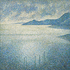
I used TF’s assign operation to set the input variables to different values. First it was set to the ‘real image’ so I could collect the response to aim for (this would be fed into the labels of the TF mean-squared-error loss). Then I set it to some white noise as this was the variable I wanted to train (the prediction output using this input would be the predictions of the loss). Wrapped up the loss in an optimizer and tried to run it… success! The loss decreased. I changed the ‘real image’ from a fake numpy array to real data and the loss still seemed to go down which was a good sign. Obviously this time the loss started a lot higher since our white noise input variable was a lot further from the real image. The white noise input variable I was optimizing came about from a numpy random array which by default gives us values between 0 and 1. I found that I could give this variable a ‘helping hand’ by multiplying it by 255 thereby making it a little closer to the real image at hand. This sped up training a little. More noticeably, the types of optimized images during training look quite different depending on which intialization method you use. The figure below showcases the images at step 0, 2500, and 5000. The top row is from a starting range between 0 and 1 while the bottom is between 0 and 255.

Another helpful change I found was to use a higher learning rate than the default. If you use the Adam optimizer, as I did, the default learning rate is 1e-3. However, I think that because here we are continuoulsy optimizing the same, small set of values, the image pixels, the learning rate should be higher. I found that 1e-1 worked fine. In the set of figures below, you can see the differences in the loss and the final image produced when using both these learning rates (smaller learning rate shown on the left):

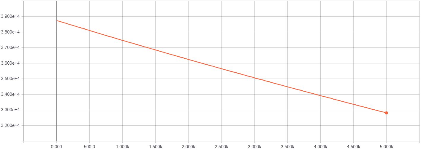
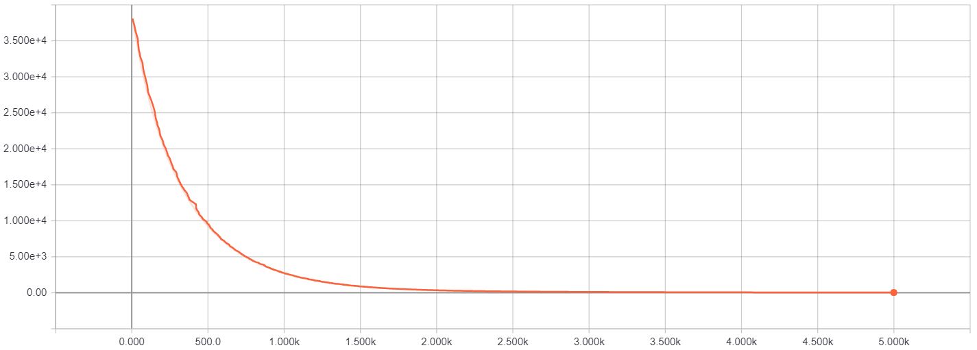
The loss y-axis doesn’t cover the same range exactly (the images are from separate Tensorboard plots). However, the axis with the smaller learning rate has a higher maximum and minimum tick which helps highlight just how slowly learning was happening. The rate of decrease is the obvious giveaway.

It’s almost never sufficient to look at the loss to determine if your model is working correctly. The great thing about working with images is that you can always visually inspect the progress along the way and it should make some sense. I viewed the optimized image at a few points during the training and realised that things weren’t quite adding up. The images I was viewing in the notebook mostly looked like noise, especially if I tried to reconstruct the image based on deeper features. However, the images I was saving to disk with OpenCV(cv2) looked much better. At the time, I put this down to a missing gap in understanding between PyPlot(plt) and notebook interactions.

I realised that I needed some heavier debugging and decided it was time to set up one of my favourite tools: Tensorboard. If you use TF, I would highly recommend using Tensorboard. Even if you’re just interested in the loss and won’t be visualizing any images along the way, use Tensorboard.

The full benefits I’ve experienced from Tensorboard is a tale for another day. To tide you over, I’ll mention briefly here how I used it.

For this project, I used Tensorboard for:

• Plotting the loss
• Viewing images throughout training
• A visual depiction of the graph

Viewing the loss was fairly straightforward in this instance since there was only one loss and it was for the same input each time. The images I saw more closely matched the images I had saved to disk rather that those I was trying to display within the notebook which was a healthy confirmation that I was probably doing the right thing. There were some slight differences between the disk and Tensorboard images which I would later figure out were due to the way I was saving images with cv2. It was definitely a bit of a gotcha. Finally, by looking at the graph, I could confirm that everything was hooked up the way I wanted it to be. One tip here is to name all your variables. I sometimes forget to do this and it comes back to bite me when I’m trying to access a particular node of a saved graph. It also makes debugging the graph slightly harder. For example, consider the two graphs below. Specific names are so much more helpful compared to generic ‘Variables’.

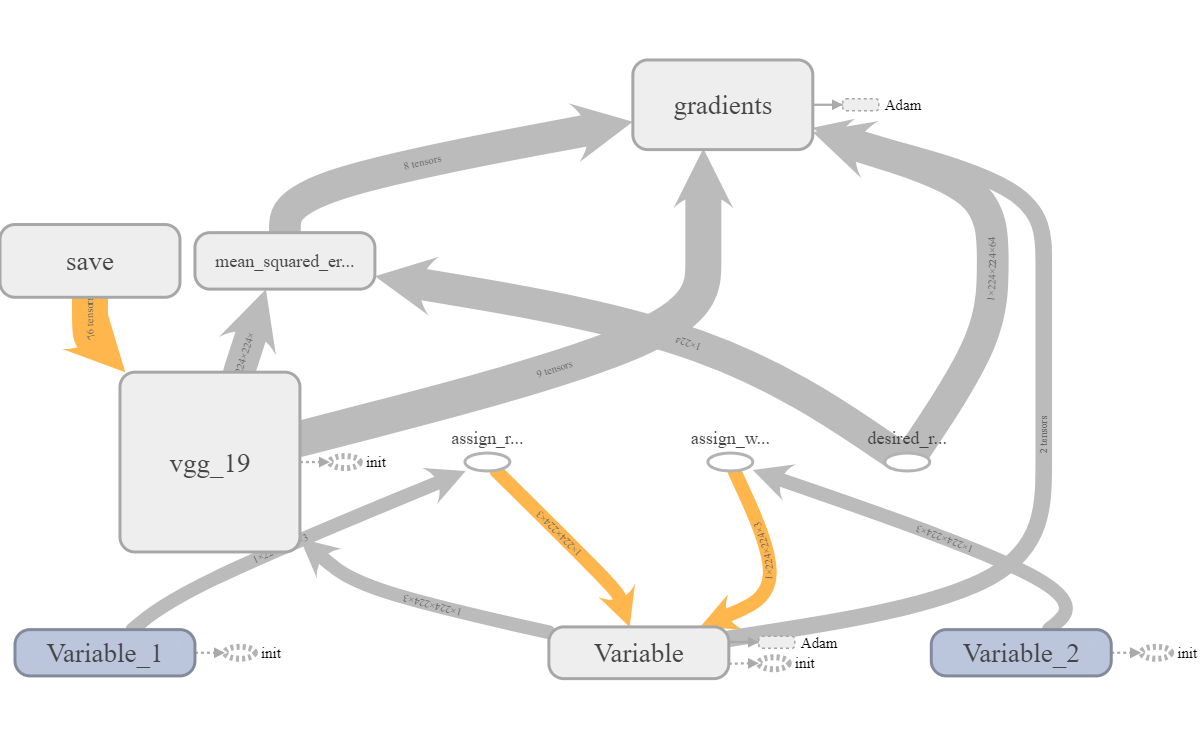
When I initially had the less helpful graph, I could still tell it was correct since the assign operations the real and white noise variables were tied to had been named. Also, the order of the suffixes matches the order the variables were created in which helps differentiate similarly named variables. Nonetheless, I reran the code with properly named variables to obtain a better good graph.

With all the connections looking fine and the image transforming as expected, I spent some time digging into the plt and cv2 libraries to make sure I could obtain the same images at a given time step for different methods: plt, cv2, and tensorboard. You can read about that here.

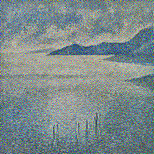
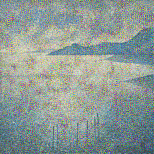
Finally, the figure below shows my notebook’s take on the images produced in the Content Reconstruction bit of Figure 1. The images from left to right are:

• Original image
• Reconstruction using conv1_2
• Reconstruction using conv2_2
• Reconstruction using conv3_2
• Reconstruction using conv4_2
• Reconstruction using conv5_2

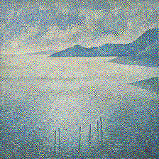
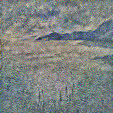
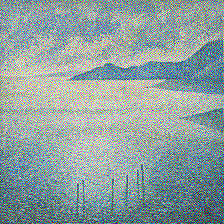
These were all obtained after 100,000 steps of training except for the conv2_2 case. That image was pulled after about 10,000 steps. As optimization for that feature layer went along, it started to pick up some odd artifacts producing the image below:

Perhaps regularization of some sort is required and I’ll look into that down the line. For the other images, 100,000 steps was probably an unnecessarily large number of steps. When you tinker around, you might find a much lower number you’re happier to work with. If so, go for it.

Overall, I probably spent about 20 hours coming up with this notebook. There were a few time consuming things that I left out (e.g. a brief dally with TF Eager, losing some unsaved work at one point and having to rewrite, blogging, …) but this post covers most of what I did. That’s it for now! Next up will be Style Representation/Reconstruction which I’ll link to once it’s up and ready!

References

[1] Gatys, L.A., Ecker, A.S. and Bethge, M., 2016. Image style transfer using convolutional neural networks. In Proceedings of the IEEE Conference on Computer Vision and Pattern Recognition (pp. 2414-2423).

• 2020 3
• 2019 3
• 2018 11