Style Reconstruction

If you’re reading this, I’m assuming that you’ve read the paper Image Style Transfer Using Convolutional Neural Networks and have some familiarity with it.

Here is the image (resized to 224x224) I’ll be working with for this post:

The focus of this post is on the Style Representation/Reconstruction section of the paper, Section 2.2 to be precise. The authors use the title Style Representation yet I’ve also included the word Reconstruction here since that’s what they did in Figure 1 and what I’ve attempted to do on my own as well. Throughout this article, I’m essentially describing building this notebook.

This post follows my previous one on the Content Representation/Reconsturction section of the paper. I’ll be making a couple of references to it and this notebook is largely based of my previous one. If you haven’t yet, I’d recommend checking out that blog post before this one.

Working through this section was a whole lot easier than the previous one. Primarily, this was because I didn’t have to deal with lots of teething issues which I’ve documented in other blog posts called gotchas (referenced throughout my previous post). The previous notebook also provided a lot boilerplate code that I could easily use here.

With that being said, I did run into some unforeseen issues, some of which I’ll talk about in this post and others, more general issues, will be covered in further gotcha posts.

So the first step in this section was coding up a function to compute the gram matrix, used in equation 3 of the paper. While it was very clear what they were doing, an efficient implementation wasn’t obvious to me until I read the description of it on Wikipedia. To summarize, you can compute the gram matrix G by V^TV where the columns of V are the vectorized feature maps for a particular layer. That was a very handy definition that saved me from trying to interpret equation 3 directly and write for loops. I also wrote a function to implement equation 4 but that was relatively straightforward. While working on these functions, I ran into a small bump regarding the use of tf.shape. You can read about that at this gotcha.

With that done, I hit the first speed-bump for this section: I wanted the number of layers used to be a parameter. When implementing the content reconstruction, the graph always had the same(ish) nodes. Yes, you chose which layer you wanted to base the reconstruction on but it was always just one layer used. With style reconstruction however, your choices were:

• Layer 1
• Layer 1, 2
• Layer 1, 2, 3
• Layer 1, 2, 3, 4
• Layer 1, 2, 3, 4, 5

So this meant that the graph would have to have a different number of nodes on different runs if the number of layers was a parameter. I didn’t want to set the graph up so that all the nodes were created and only the relevant one were used depending on the parameter’s setting: don’t create nodes you don’t need. The solution was quite simple: for loops. I used for loops to generate the nodes as required. In hindsight, this was as easy as it sounds. I think the big block for me was simply that I hadn’t done this before. I was used to creating graphs in a very static manner, knowing beforehand exactly what the graph consisted of and the graph having the same number of nodes for different runs.

This did make the graph a little harder to understand when more layers were used. In the figure below, the image on the left uses 2 layers and the one on the right, 5 layers:

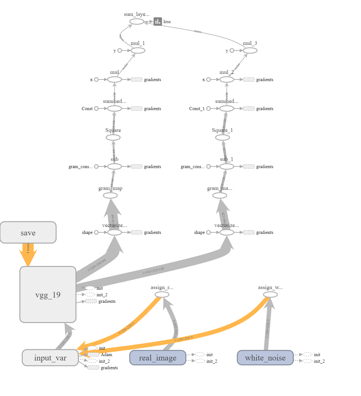
You can see that with 5 nodes, tensorboard simply collapsed similar information but this concise view isn’t great for debugging.

Working in the 2 layer setting, I ensured that the connections worked as intended and assumed that the same would hold for 5. For the majority of the implementation, I used the settings with 1 layer and 2 layers to check that the implementation was working. Just using the 1 layer setting would have been insufficient because perhaps there was a bug that only showed when the loop tried to run again. Conversely, just using 2 wouldn’t have been enough either because there could have been some edge cases that didn’t handle lists of size 1.

Given that I was now working with a graph with a variable number of nodes, the next tricky bit that arose was how to handle the placeholders for the loss computation. Previously when implementing the content reconstruction, the loss was computed between the output of the graph on the image being optimized and the features of the content image. There was always just a single placeholder for the latter. If I wanted to use the same methodology here, I would have to find a way of having a variable size feed_dict. While this may be possible, I didn’t know exactly how to do it. So I made a switch which in hindsight, seems a lot cleaner than my previous approach and really I should have used it even with the content reconstruction: replacing the placeholder(s) with constant(s).

The information I required for the loss were the gram matrices of the style image. This information would never change so really it could be a constant. I was just used to the idea of having at least one tensor being fed via a placeholder when it came to evaluating and running a graph so I shoehorned the feature representation into this roll when implementing the content reconstruction. I could get away with it there since there was only ever 1 placeholder.

In this instance, I ran the graph on the style image, obtained the gram matrices, and assigned them to constants, stored in a list. I then ran the graph on the image being optimized and collected the gram matrices to be stored into another list. Given these two lists, it was fairly straightforward to compute the loss.

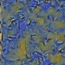
Using just the first 2 layers, here is one of the first reconstructions I obtained using coastal scene as my style image:

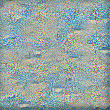
At best, underwhelming, at worst, incorrect. Honestly, I couldn’t quite be sure if the process was working or broken.

I’ve stared at the original image, and images like it, many times such that I have developed a very specific idea of its style; I was not seeing this idea being borne out in the reconstruction. I associate this painting with pointillism so I expected the style image to consist of a lot of more … points. However, setting aside my beliefs about this image’s style, I have to consider what the network is built to do. As we go deeper within the network, fine-grained detail such as the individual points of paint that make up the image are lost as focus is shifted to more abstract concepts. So in this case, we move from dotted points of blue and white to patches of white surrounded by blue. Looking at both the maths of the network and the image itself, I can see where the optimized image is coming from.

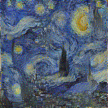
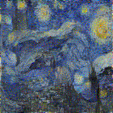
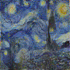
Though if I being completely honest, I only came to this conclusion later on down the pipeline after franctically investigating another avenue: what do my reconstructions look like if I compare them to what was in the paper? I switched to using starry night as the style image and carried out style reconstruction with 2 layers:

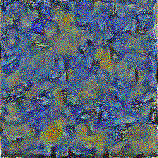
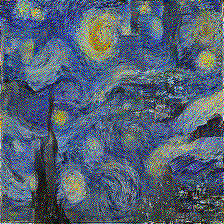
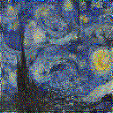
I can see some similarities but also a lot of differences. Looking at the original work, the reconstruction using 5 layers seemed to have the most global coherence to me so I tried with 5 layers:

This match was a lot closer to what was in the paper but I still had some concerns. In the paper, they stated that the style reconstructions discarded information regarding the global arrangement but in my reconstruction, there still seemed to be too much structure. The only remaining difference I could see between my implementation and the paper was the size of the reconstructions: I was working with 224x224 whereas the paper had 512x512. I sought to rectify this.

Two issues arose when I went down this route. Initially when I changed the height and width in the notebook, I received an error because the new tensor shape wasn’t compatible with the tf.squeeze operation being carried out in the vgg_19 implementation provided by TF. The easy immediate fix was to simply remove this line since I was not using that endpoint from the network but I took it one step further. For this work, only the first few endpoints provided by the vgg_19 function are required so I created a new function that only contained these relevant endpoints. If you won’t use the endpoints, don’t clutter the graph with them.

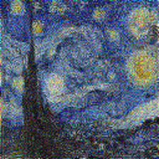
With this change in place, I obtained the reconstructions using 1 and 2 layers:

They seemed the same as what I was acheiving before, simply on a larger scale. I then increased the number of layers to 5, ran the notebook, and … my computer restarted (herein rose the second issue). After a few more attempts at this, each of which restarted my computer without fail, I realised that I had hit a hardware bottleneck. My GPU of 8Gb didn’t have enough memory to hold the information when using 512x512 with 5 layers. While this would normally just result in a TF OOM error, my aging and tempremental power supply cuts out whenever the GPU tries to draw a bit more than usual. So 512x512 images with 5 layers was off the table with my meagre resources. 4 and 3 layers were also too many to handle.

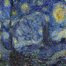
Here’s what the previous 512x512 reconstructions look like compared to their 224x224 counterparts:

512x512 is shown on the left, 224x224 on the right, the first row uses 1 layer and the second, 2 layers. For the purpose of displaying them here, I resized the 512x512 image to be 224x224 after the reconstruction. There’s no surprising difference between them really. As one might expect, the 224x224 versions simply look like zoomed in versions of the 512x512. In fact, I can take a random 224x224 crop of the 512x512 image to enhance the similarity:

Still I wasn’t convinced so I took two more steps:

• Reconstructing using different sizes (128x128, 176x176, 224x224, 512x512).
• Changing the initial seed (0, 1, 2).

Once again, for the purposes of display, everything has been resized to 224x224.

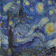
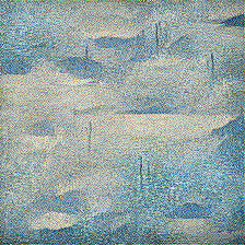
First, let’s examine the reconstructions using 224x224 and all 5 layers. The columns correspond to the different seeds:

The amount of localization does seem to vary quite a bit depending on the seed. This confirmed my hunch that the initialization point for the image does play an important role. Not so much for providing a ‘correct’ output but for providing output that ‘looks’ better. In this case, looking better to me meant less global arrangement.

Next, using 5 layers, here’s how using different sizes affected the outcome (from left to right: 128, 176, 224; from top to bottom: seeds 0, 1, 2):

There weren’t too many differences. The obvious quality in difference is due to the resolution.

There are still some differences compared to what the paper shows but I do not think these are due to major inaccuracies in the implementation. I think the smoother look in the paper is from using a higher resolution and perhaps there were some tricks employed in the optimization procedure that they neglected to mention.

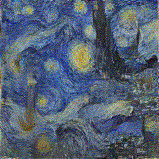
Still these results with starry night were sufficient to convince me to try the procedure on coastal scene. Using 224x224, the number of layers increases from 1 to 5 as we move left to right:

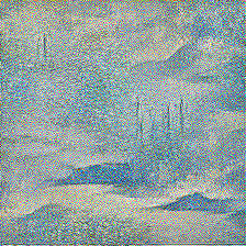
For all choices of layers, I tried 3 seeds and what’s shown above is what appealed to me the most.

I think my idea of style for coastal scene is definitely a lot more localized. I would say that here using just 1 layer reconstructs the image with the most distilled essence of style. Perhaps if I wish to transfer the pointilism style of coastal scene onto another image, I shouldn’t use all 5 layers for the style. However, it’s clear that when using more layers, the network is trying to capture the image from a higher vantage point, considering more of the image, and the individual points of paint do not play as big a role.

I managed to achieve my initial goal: recreate the style reconstruction images in the original paper as applied to coastal scene. That brings this blog to a close. Keep an eye out for the third and final installment where I bring together content and style reconstruction to properly transfer the style of one image onto another!

P.S.

Before resizing, the original coastal scene image I had was 800x662:

So you don’t have to scroll all the way back up, the 224x224 version looks like this:

The difference is quite obvious. It’s unfortunate that my hardware bottleneck prevented me from using a higher resolution. The pointilism style is a lot more obvious at a higher resolution. When compressed, the points blur and we are left with less-appealing squares. As part of the pointilism technique, the viewer is supposed to blur the various points together so that they meld together when viewed at a distance. Having the image do the blurring for you, and not very well at that, is very underwhelming.

I take solace in this: even if it was a higher resolution, it wouldn’t be enough. I have a more detailed copy sitting on my desk and yet it’s still insufficient. When moving from the 3D of canvas and paint to the (essentially) 2D of a computer printed image, a lot is lost.

References

[1] Gatys, L.A., Ecker, A.S. and Bethge, M., 2016. Image style transfer using convolutional neural networks. In Proceedings of the IEEE Conference on Computer Vision and Pattern Recognition (pp. 2414-2423).

• 2020 3
• 2019 3
• 2018 11